Fare Prediction
Motivation
We wanted to look at what variables were significant predictors for fare, with the final goal of building a taxi fare estimator that could take values on these selected key variables and produce an estimated fare for users, together with a 95% prediction interval.
Exploratory graphs
First, we did some exploratory analysis to provide a brief overview on the outcome variable fare, and how it was distributed across boroughs, neighborhoods, type of taxis, and time of day.
We can see that the highest total fares were observed during morning rush hours (6-9am), evening rush hours (4pm-6pm), dinner time (6pm-9pm), and tapering off a little at night (after 9pm) on Valentine’s Day. This high amount of aggregate fares show that people either traveled in high volumes to drop-off locations in Manhattan, or took longer trips from other boroughs to Manhattan (longer distance travelled) during these hours. Furthermore, yellow taxis constituted the most rides, which suggested that these trips took place mostly below East 96th and West 110th Street.You might also be interested in the neighborhoods in Manhattan with the highest average taxi fares (which suggests they are popular (or maybe they’re just far from downtown!) If so, you can check it out in the Shiny app!
The distribution of the outcome variable, fare amount, can be found below. 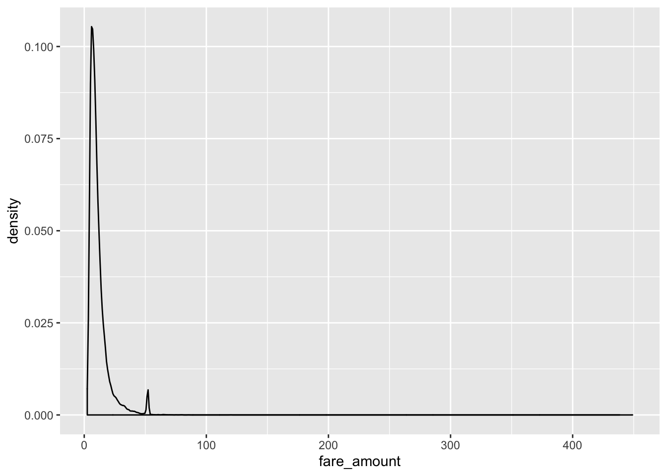
Since the data looked heavily right skewed, we decided to drop fares that are above $60, based on our assumption that most of the fares above 60 were mostly negotiated fares.
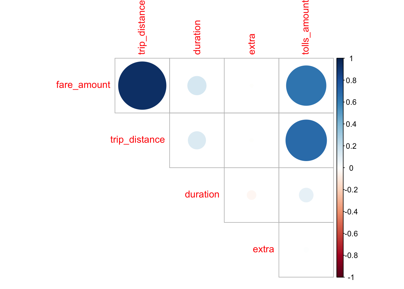
Qualitatively, the variables that might be reasonably associated with fare amount include: trip duration, trip distance, time of day, tolls amount, taxi type, pick-up borough, and extra fees. So a regression model with the abovementioned as predictors can be our original expanded model. However, it might also be a good idea to look at the correlation plot between fare and other continuous variables.
Model Building
Looking at the correlation plot, we saw that outcome variable fare was highly correlated with trip distance and tolls amount, as well as duration, so we included these as predictors for our second model. Qualitatively, we also added time of day to this model.
We also used stepwise regression with AIC as the criterion to potentially get a more parsimonious model. Stepwise regression did not suggest leaving any variables out of the model (stick with the original expanded model). However, we wanted to see if a very parsimonious models (only with trip distance and duration as predictors) would perform better.
Next, we fitted the expanded model, as the stepwise regression result suggested. Model diagnostics suggested that observation 123 and 16214 were highly influential points (based on crossing Cook’s distance cut-off value), so we removed those.
We refitted the model, and below is the stepwise regression summary output for this first model.
| term | estimate | std.error | statistic | p.value |
|---|---|---|---|---|
| (Intercept) | 3.8684367 | 0.3042991 | 12.712614 | 0.0000000 |
| trip_distance | 2.9118704 | 0.0105459 | 276.113652 | 0.0000000 |
| duration | 0.0026267 | 0.0002564 | 10.244701 | 0.0000000 |
| as.factor(time_of_day)early morning | -1.0207754 | 0.1566061 | -6.518105 | 0.0000000 |
| as.factor(time_of_day)morning rush | 0.8995413 | 0.0653084 | 13.773748 | 0.0000000 |
| as.factor(time_of_day)others | 1.6313873 | 0.0613872 | 26.575351 | 0.0000000 |
| as.factor(time_of_day)lunch | 1.6366897 | 0.0755285 | 21.669832 | 0.0000000 |
| as.factor(time_of_day)evening rush | 1.3087173 | 0.0704371 | 18.579935 | 0.0000000 |
| as.factor(time_of_day)dinner time | 0.4881317 | 0.0648335 | 7.529000 | 0.0000000 |
| extra | 0.0418498 | 0.0143383 | 2.918741 | 0.0035176 |
| tolls_amount | 0.3184096 | 0.0346663 | 9.184997 | 0.0000000 |
| as.factor(type)yellow | 0.1630431 | 0.0763189 | 2.136341 | 0.0326613 |
| as.factor(pu_boro)Brooklyn | 0.8848642 | 0.3345617 | 2.644846 | 0.0081779 |
| as.factor(pu_boro)Manhattan | -0.4008831 | 0.2996303 | -1.337926 | 0.1809328 |
| as.factor(pu_boro)Queens | -2.6402839 | 0.3276419 | -8.058443 | 0.0000000 |
| r.squared | adj.r.squared |
|---|---|
| 0.8806238 | 0.8805572 |
Fitting the most parsimonious model (with duration and distance as predictors) gave the regression outputs below:
| term | estimate | std.error | statistic | p.value |
|---|---|---|---|---|
| (Intercept) | 4.6918487 | 0.0234144 | 200.38332 | 0 |
| trip_distance | 2.8695304 | 0.0067880 | 422.73319 | 0 |
| duration | 0.0028756 | 0.0002572 | 11.18014 | 0 |
| r.squared | adj.r.squared |
|---|---|
| 0.8748377 | 0.8748281 |
And below is the “moderate” model (with duration and distance as predictors) and its regression outputs:
| term | estimate | std.error | statistic | p.value |
|---|---|---|---|---|
| (Intercept) | 3.7237533 | 0.0532879 | 69.879943 | 0 |
| trip_distance | 2.8929383 | 0.0068470 | 422.511520 | 0 |
| duration | 0.0026141 | 0.0002574 | 10.157020 | 0 |
| as.factor(time_of_day)early morning | -1.0635439 | 0.1572182 | -6.764762 | 0 |
| as.factor(time_of_day)morning rush | 0.8860394 | 0.0650083 | 13.629643 | 0 |
| as.factor(time_of_day)others | 1.6079726 | 0.0613598 | 26.205621 | 0 |
| as.factor(time_of_day)lunch | 1.6095612 | 0.0754878 | 21.322144 | 0 |
| as.factor(time_of_day)evening rush | 1.3060180 | 0.0701718 | 18.611727 | 0 |
| as.factor(time_of_day)dinner time | 0.4814640 | 0.0650064 | 7.406410 | 0 |
| r.squared | adj.r.squared |
|---|---|
| 0.8795327 | 0.8794943 |
Cross-validation
Now, we have 3 models that we wanted to cross-validate and compare cross-validated prediction error RMSE.
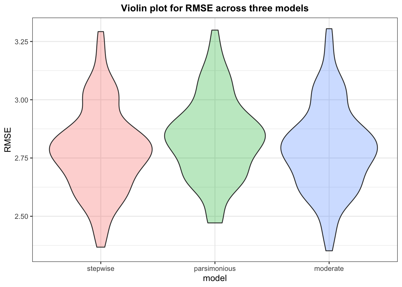
This plot above suggests that although the moderate model performs only marginal better than the stepwise and parsimonious model, it seems to be the best choice given a balance of both parsimony and better predictive ability. This model also has an R-squared of 88%.
Check for multicollinearity
| GVIF | Df | GVIF^(1/(2*Df)) | |
|---|---|---|---|
| trip_distance | 1.019654 | 1 | 1.009779 |
| duration | 1.017731 | 1 | 1.008827 |
| as.factor(time_of_day) | 1.003549 | 6 | 1.000295 |
Since VIF for all predictors are below 5, we don’t need to worry about multicollinearity.
In the end, we decided to go with the model below for fare prediction:
\(\hat{Fare} = \hat{\beta_{0}} + \hat{\beta_{1}} \times Duration + \hat{\beta_{2}} \times Distance + \hat{\beta_3} \times I(time of day = early morning) + \hat{\beta_4} \times I(time of day = morning rush) +\) \(\hat{\beta_5} \times I(time of day = lunch) + \hat{\beta_6} \times I(time of day = evening rush) + \hat{\beta_7} \times I(time of day = dinner time) + \hat{\beta_8} \times I(time of day = night)\)
Fare prediction
The data only has fare and duration data for taxi’s, so we only looked at Yellow and Green taxi’s observations (whose fares are at most $60 and excluding trips in Staten Island).
We used the model obtained above to create a Shiny app that helps predict taxi fare based on the three predictors in the final selected model:
Distance (in miles) – variable “trip_distance” in the dataset
Duration (in minutes) – new variable created by taking the time difference between “pick-up time” and “drop-off time”
Time of day – we categorized this continuous variable into a factor with 6 levels that might sound more intuitive. Specifically, they are:
6am-9am: morning rush
11am-1pm: lunch
4pm-6pm: evening rush
6pm-9pm: dinner time
9pm-12am and 12am-2am: night
9am-11am and 1pm-4pm: others
Please feel free to use the app here to see how much it might cost you to travel from your current neighborhood to your desired neighborhood!
(Note that this inference might only be valid for Valentine’s Day and for prices that are less than $60)